# 基于求解器的投资组合优化问题的二次规划
说明关于基本投资组合模型的基于求解器的二次规划的示例。
此示例说明如何使用 quadprog 中的内点二次规划算法来求解投资组合优化问题。函数 quadprog 属于 Optimization Toolbox。
在此示例中定义问题的矩阵是稠密矩阵;然而,quadprog 中的内点算法也可以利用问题矩阵的稀疏性来提高速度。
# 二次模型
假设存在
令
经典的均值-方差模型是在一组约束条件下最小化投资组合风险,风险可由下式衡量:
其中约束如下:
预期回报率不应低于投资者期望的最低投资组合回报率
, 投资组合比例
的总和应为 1, 而且作为比例(或百分比),它们应为介于 0 和 1 之间的数字,
由于最小化投资组合风险的目标函数是二次型的,而约束是线性的,因此该优化问题是二次规划,即 QP。
# 225 项资产问题
现在让我们求解包含 225 项资产的 QP。该数据集来自 OR-Library [Chang, T.-J., Meade, N., Beasley, J.E. and Sharaiha, Y.M., "Heuristics for cardinality constrained portfolio optimisation" Computers & Operations Research 27 (2000) 1271-1302]。
我们加载数据集,然后按 quadprog 所需的格式设置约束。在此数据集中,回报率
加载存储在 MAT 文件中的数据集。
using TyOptimization
using TyMath
using TyPlot
using TyBase
path = pkgdir(TyOptimization)
data = load(path * "/data/port5.mat")
基于相关矩阵计算协方差矩阵。
Covariance = Correlation .* (stdDev_return * stdDev_return');
nAssets = length(mean_return); r = 0.002;     # number of assets and desired return
Aeq = ones(1,nAssets); beq = 1;              # equality Aeq*x = beq
Aineq = -mean_return'; bineq = -r;           # inequality Aineq*x <= bineq
lb = zeros(nAssets,1); ub = ones(nAssets,1); # bounds lb <= x <= ub
c = zeros(nAssets,1);                        # objective has no linear term; set it to zero
# 在 Quadprog 中选择内点算法
为了使用内点算法求解 QP,我们将选项算法设置为 'interior-point-convex'。
options = optimoptions(:quadprog,Algorithm = "interior-point-convex");
# 求解 225 项资产问题
我们现在设置一些额外的选项,并调用求解器 quadprog。
设置附加选项:打开迭代输出,并设置更严格的最优性终止容差。
options = optimoptions(options,Display = "iter");
调用求解器并测量挂钟时间。
@time x1,fval1 = quadprog(Covariance,vec(c),Aineq,[bineq],Aeq,[beq],vec(lb),vec(ub),[],options);
Iter            Fval   Primal Infeas     Dual Infeas   Complementarity
   0    7.212813e+00    1.975147e+03    2.230265e-01      2.121324e+01
   1    5.087187e-04    1.360917e+00    1.536699e-04      2.830551e+00
   2    3.936395e-04    8.181869e-01    9.238672e-05      4.511132e+00
   3    3.525742e-04    2.468966e-01    2.787868e-05      7.635321e-01
   4    5.519330e-04    1.234483e-05    1.393936e-09      1.487781e+00
   5    5.519320e-04    1.923520e-09    2.455588e-13      2.376074e-04
   6    4.680051e-04    3.926649e-10    5.012570e-14      7.796372e-05
   7    3.606961e-04    1.377623e-11    1.753372e-15      1.406325e-05
   8    2.982304e-04    1.989739e-14    3.686287e-18      1.085233e-05
   9    2.729816e-04    1.874721e-14    2.493665e-18      4.602483e-06
  10    2.238534e-04    1.014434e-14    5.854692e-17      4.445010e-05
  11    2.099378e-04    1.628271e-14    2.818926e-18      6.357395e-06
  12    1.971963e-04    1.986036e-14    1.246832e-18      7.627446e-07
  13    1.952795e-04    1.820585e-14    8.673617e-19      3.467287e-08
  14    1.949127e-04    1.989459e-14    1.002887e-18      1.305679e-10

Minimum found that satisfies the constraints.

Optimization completed because the objective function is non-decreasing in feasible directions, to within the value of the optimality tolerance and constraints are satisfied to within the value of the constraint tolerance.

  0.282460 seconds (5.12 k allocations: 64.743 MiB, 12.99% gc time)
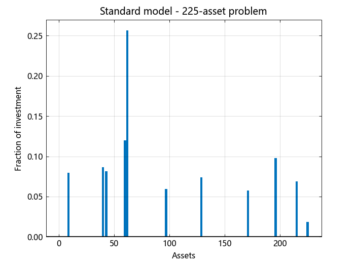
绘制结果。
bar(x1,width = 2)
ylabel("Fraction of investment")
xlabel("Assets")
title("Standard model - 225-asset problem")
grid("on")
# 具有组约束的 225 项资产问题
我们现在向模型增加一组约束,即要求投资者 30% 的资金必须投资于资产 1 至 75,30% 投资于资产 76 至 150,30% 投资于资产 151 至 225。每组资产可以是不同行业,例如技术、汽车和制药。
实现此新要求的约束为:
向现有等式约束添加这组不等式约束。
Groups = blkdiag(ones(1,div(nAssets,3)),ones(1,div(nAssets,3)),ones(1,div(nAssets,3)));
Aineq = [Aineq; -Groups];         # convert to <= constraint
bineq = [bineq; -0.3*ones(3,1)];  # by changing signs
调用求解器并测量挂钟时间。
@time x2,fval2 = quadprog(Covariance,vec(c),Aineq,vec(bineq),Aeq,[beq],vec(lb),vec(ub),[],options);
Iter            Fval   Primal Infeas     Dual Infeas   Complementarity
   0    7.212813e+00    2.304305e+03    5.062751e+00      2.598079e+01
   1    5.014626e-04    1.446136e+00    3.177280e-03      3.299995e+00
   2    4.043363e-04    8.119089e-01    1.783832e-03      2.442291e+00
   3    3.474328e-04    2.375218e-01    5.218552e-04      1.628265e+00
   4    3.829175e-04    1.187609e-05    2.609276e-08      3.536073e-01
   5    3.829158e-04    1.191021e-09    2.628376e-12      3.943413e-05
   6    3.536513e-04    2.790679e-10    6.158524e-13      1.232625e-05
   7    2.965677e-04    2.469723e-11    5.447932e-14      5.401752e-06
   8    2.621091e-04    1.974690e-14    7.209944e-18      2.979064e-06
   9    2.234785e-04    1.310451e-14    2.276825e-18      5.842570e-06
  10    2.082052e-04    1.542020e-14    1.084202e-18      1.104407e-06
  11    2.027746e-04    1.886318e-14    2.114194e-18      3.336141e-08
  12    2.009830e-04    2.021292e-14    9.486769e-19      1.646531e-09

Minimum found that satisfies the constraints.

Optimization completed because the objective function is non-decreasing in feasible directions, to within the value of the optimality tolerance and constraints are satisfied to within the value of the constraint tolerance.

  0.240488 seconds (5.03 k allocations: 62.282 MiB, 6.91% gc time)
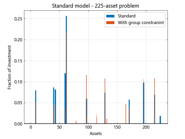
绘制结果,叠加在先前问题的结果上。
hold("on")
bar(x2)
legend(["Standard","With group constranint"])
hold("off")
# 迄今为止结果摘要
我们从第二个条形图中看到,由于存在额外的组约束,与第一个投资组合相比,现在投资组合在三个资产组中的分布更均匀。这种强加的多样化也导致风险略微增加,这是通过目标函数来测量的(请参阅两次运行的迭代输出中最后一次迭代的标记为“f(x)”的列)。
# 使用随机数据的 1000 项资产问题
为了说明 quadprog 的内点算法如何处理更大型的问题,我们将使用包含 1000 项资产的随机生成的数据集。
重置随机流以实现可再现性。
rng = MT19937ar(0);
nAssets = 1000; # desired number of assets
生成 -0.1 到 0.4 之间的回报率均值数据。
a = -0.1; b = 0.4;
mean_return = a .+ (b-a).*rand(rng,nAssets,1);
生成 0.08 到 0.6 之间的回报率标准差数据。
a = 0.08; b = 0.6;
stdDev_return = a .+ (b-a).*rand(rng,nAssets,1);
# Correlation matrix, generated using Correlation = gallery('randcorr',nAssets).
# (Generating a correlation matrix of this size takes a while, so we load
# a pre-generated one instead.)
path = pkgdir(TyOptimization)
data = load(path * "/data/correlationMatrixDemo.mat")
# Calculate covariance matrix from correlation matrix.
Covariance = Correlation .* (stdDev_return * stdDev_return');
# 定义并求解随机生成的 1000 项资产问题
我们现在定义标准的 QP 问题(此处没有组约束)并求解。
r = 0.15;                                     # desired return
Aeq = ones(1,nAssets); beq = [1];               # equality Aeq*x = beq
Aineq = -mean_return'; bineq = [-r];            # inequality Aineq*x <= bineq
lb = zeros(nAssets); ub = ones(nAssets);  # bounds lb <= x <= ub
c = zeros(nAssets);                         # objective has no linear term; set it to zero

@time x3, = quadprog(Covariance,c,Aineq,bineq,Aeq,beq,lb,ub,[],options);
Iter            Fval   Primal Infeas     Dual Infeas   Complementarity
   0    2.144124e+01    1.306964e+04    2.686312e+00      4.519961e+01
   1    9.603334e-02    1.156196e+02    2.376427e-02      5.507976e+00
   2    9.472022e-05    9.980635e-01    2.051404e-04      9.096405e-02
   3    7.912080e-05    4.990318e-05    1.025702e-08      1.035340e-03
   4    7.905810e-05    2.067984e-08    4.250529e-12      1.123253e-06
   5    3.353342e-05    2.173559e-10    4.471614e-14      4.747129e-07
   6    1.856073e-05    6.550039e-14    1.111307e-17      4.743841e-07
   7    1.458766e-05    8.263706e-14    2.289530e-18      2.539410e-08
   8    1.371413e-05    8.318969e-14    9.911344e-19      9.405355e-10

Minimum found that satisfies the constraints.

Optimization completed because the objective function is non-decreasing in feasible directions, to within the value of the optimality tolerance and constraints are satisfied to within the value of the constraint tolerance.

  2.605711 seconds (15.60 k allocations: 722.423 MiB, 2.48% gc time)