2026a

# Julia 高性能编程

# 概述

Julia 是一门灵活的动态语言，适合用于科学计算和数值计算，并且性能可与传统的静态类型语言媲美。写出能用的 Julia 代码很容易，但写出高性能的 Julia 代码则需要一定的知识储备。本文主要从 6 个方面、总结了 31 条高性能编程经验，帮助用户写出高性能代码。

# 核心思路

检查性能热点
常见性能优化
- 避免全局变量
- 避免不必要的数据计算
- 基于多重派发的特定优化
类型稳定优化
- 确保类型稳定
- 确保结构体或矩阵的元素类型是具体类型
内存优化
- 预分配
- 使用视图
- inplace 原地操作
循环优化
- 按内存排列顺序访问数组
- @simd 和 @inbounds 加速
- 多线程加速
合理使用广播和向量化编程
使用高效的算法和数据结构

# 检查性能热点

针对工程的性能优化，首先需要检查性能热点，然后想办法优化它。

一般而言，有以下几种方法确定一个函数的性能热点：

使用 @time 或者 BenchmarkTools 提供的 @btime 宏来检查某些片段的执行时间
通过@profview宏以可视化的方式将性能采样结果与代码行绑定在一起

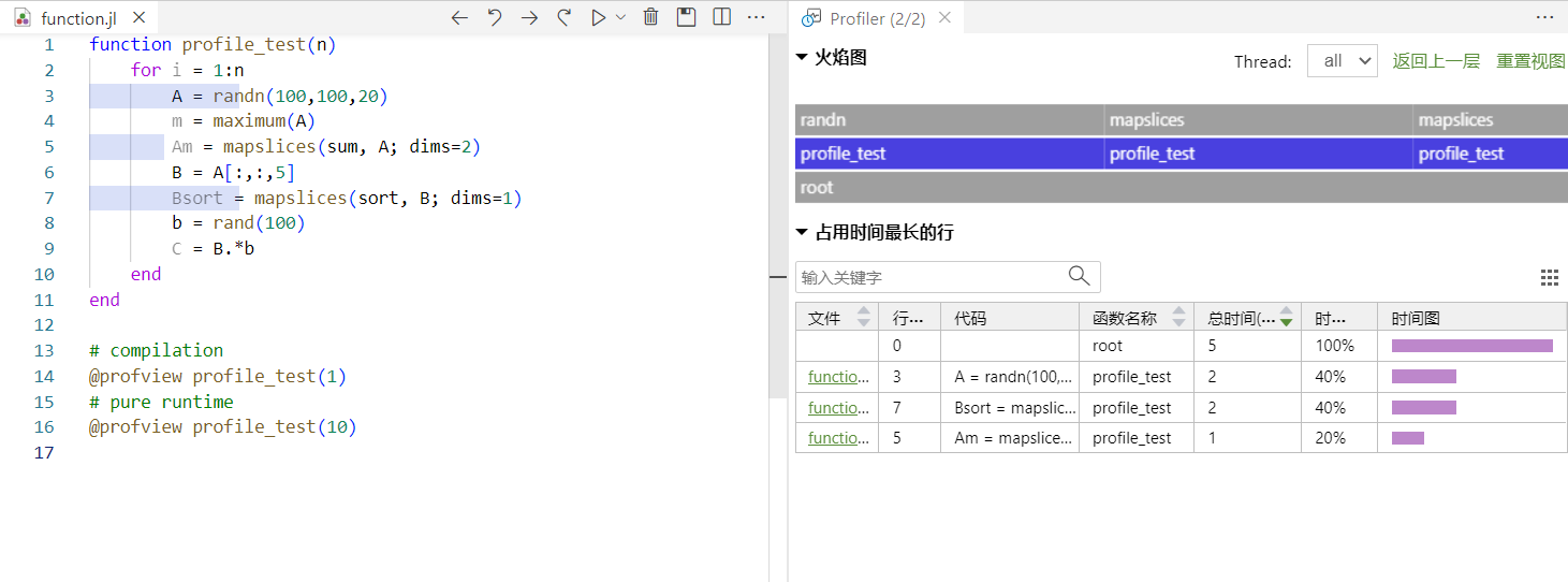
关于性能分析工具的使用，可以查阅 Syslab 帮助中的 “Syslab > Syslab 环境基础知识 > 性能分析” 章节。

# 常见性能优化

# 避免全局变量

全局变量的值和类型随时都会发生变化，这使编译器难以优化使用全局变量的代码。

# bad：采用全局变量
global g_x = 1000
function f_global()
    s = 0.0
    for i in 1:g_x
        s += i
    end
    return s
end

变量应该是局部的，或者尽可能作为参数传递给函数。

# good：采用参数传递
function f_local(x::Int)
    s = 0.0
    for i in 1:x
        s += i
    end
    return s
end

如果确实需要使用全局变量，可以将其改为常量+引用。这样既保持常量特性，又允许修改其值，如DEFAULT_X[] = 3。

# good：采用常量
const DEFAULT_X = Ref(1000)
function f_const()
    s = 0.0
    for i in 1:DEFAULT_X[] # []表示解引用
        s += i
    end
    return s
end

三者性能对比如下，其中局部变量性能最好，全局变量性能最差。

using BenchmarkTools
@btime f_global() # 46.200 μs (2979 allocations: 62.19 KiB)
@btime f_local(1000) # 823.944 ns (0 allocations: 0 bytes)
@btime f_const() # 829.487 ns (0 allocations: 0 bytes)

# 避免不必要的数据计算

避免不必要的数据计算，可以大幅提升代码性能。

例如，以下代码表面看起来并没有冗余计算。

using TyMath
A = rand(1000, 1000)
B = rand(1000, 1000)
C = rand(1000, 1000)

# bad
function f_bad(A,B,C)
    for i = 1:10
        res1 = A \ B
        res2 = A \ C
    end
end

但是，仔细分析发现，对A矩阵求逆，实质是重复计算。为了避免重复计算，改造如下：

# good
function f_good(A,B,C)
    invA = inv(A) # 对 A 求逆
    for i = 1:10
        res1 = invA * B
        res2 = invA * C
    end
end

两者性能相差较大：

using  BenchmarkTools
@btime f_bad(A,B,C)  # 657.330 ms (100 allocations: 305.33 MiB)
@btime f_good(A,B,C) # 218.279 ms (45 allocations: 160.71 MiB)

# 避免不必要的字符串传递

避免冗余判断逻辑和不必要的字符串传递，提高代码性能与可读性。

下面这段代码时一个很典型的 MATLAB 风格的写法，但是在 Julia 中，这种写法不推荐：

# bad
function f_bad(op::String, A::AbstractMatrix, x::AbstractVector)
    if lowercase.(op) == "mtimes"
        y = A * x
    elseif lowercase.(op) == "mldivide"
        y = A \ x
    else
        error("Invalid op: $op")
    end
end

字符串的处理和检查本身具有额外的开销，可以直接传递运算符而非字符串：

# good
function f_good(op, A, x)
    if op in (*, \)
        return op(A, x)
    else
        error("Invalid op: $op")
    end
end

两者性能对比：

using BenchmarkTools
A = rand(2,2)
x = rand(2)
@btime f_bad("mtimes", A, x) # 144.208 ns (4 allocations: 200 bytes)
@btime f_good(*, A, x) # 66.973 ns (1 allocation: 80 bytes)

如果遇到无法传递运算符的情况，也可以使用Symbol来代替字符串：

# good
function f_other(op::Symbol, A::AbstractMatrix, x::AbstractVector)
    if op == :mtimes
        y = A * x
    elseif op == :mldivide
        y = A \ x
    else
        error("Invalid op: $op")
    end
end
@btime f_other(:mtimes, A, x) # 69.672 ns (1 allocation: 80 bytes)

# 避免 I/O 中的字符串插值

将数据写入到文件（或其他 I/O 设备）中时，生成额外的中间字符串会带来开销。

a = "the value  is"
b = 1+2im

using  BenchmarkTools

io = IOBuffer()
@btime println(io, "$a $b"); # 785.393 ns (10 allocations: 392 bytes)

io = IOBuffer()
@btime println(io, a, " ", b); # 467.347 ns (8 allocations: 288 bytes)

# 分离核心函数

许多函数遵循这一模式：先执行一些设置工作，再通过多次迭代来执行核心计算。如果可行，将这些核心计算放在单独的函数中是个好主意。例如，以下函数返回一个数组，其类型是随机选择的。

# bad
function strange_twos(n)
    a = Vector{rand(Bool) ? Int64 : Float64}(undef, n) # a 的类型是随机选择的
    for i = 1:n
        a[i] = 2
    end
    return a
end

建议改为：

function fill_twos!(a)
    for i = eachindex(a)
        a[i] = 2
    end
end;

# good
function strange_twos_fast(n)
    a = Vector{rand(Bool) ? Int64 : Float64}(undef, n)
    fill_twos!(a) # 分离核心函数，更利于优化
    return a
end;

using BenchmarkTools
@btime strange_twos(30) # 557.143 ns (1 allocation: 304 bytes)
@btime strange_twos_fast(30) # 217.635 ns (1 allocation: 304 bytes)

Julia 的编译器会在函数边界处针对参数类型特化代码，因此在原始的实现中循环期间无法得知a的类型（因为它是随机选择的）。于是，第二个版本通常更快，因为对于不同类型的a，内层循环都可被重新编译为fill_twos!的一部分。

# 基于多重派发的特定类型优化

Julia 函数 (function) 由多个方法 (method) 共同定义，多重派发调用最匹配的方法定义。Julia 多重派发围绕输入的类型构建了不同的代码实现，Julia 的代码语义由类型来承载。通过多重派发可以实现特定类型的优化实现。

假设存在一个 512x512 的对角矩阵，如果按一般矩阵处理，性能如下：

using LinearAlgebra

function mysum(A)
    rst = zero(eltype(A))
    @simd for i in eachindex(A)
        rst += A[i]
    end
    return rst
end

using BenchmarkTools

Xd = Diagonal(rand(512)) # 对角矩阵
@btime mysum(Xd) # 333.100 μs (1 allocation: 16 bytes)

Julia 的多重分派，允许我们告诉 Julia 编译器更多信息。因此，针对Diagonal类型进行特定优化，可以大幅提升性能。

# 在原先代码基础上，新增对 Diagonal 类型的特定优化
mysum(Xd::Diagonal) = mysum(Xd.diag)
@btime mysum(Xd) # 43.030 ns (1 allocation: 16 bytes)

# 类型稳定优化

# 编写类型稳定的函数

Julia 代码编译期间只能够获得类型信息，而无法获得值信息。

类型稳定的理解：

理解 1：函数的返回值类型在不同情况下是不变的
理解 2：函数的返回值（及中间结果）类型可以通过函数输入的类型来唯一推断

类型稳定的检测：

使用 @code_warntype 来验证类型不稳定行为

类型不稳定会导致：

Julia 编译器难以做充足的编译优化
额外的运行时类型检查和开销
类型不稳定往往影响的是函数调用者的性能

高性能编程建议：

尽量避免类型不稳定的代码
类型稳定不是通过过度添加类型标记来实现的，而是通过函数的合理拆分与设计
在进行任何其他性能优化之前优先评估代码类型不稳定对性能的影响
Union-Split 会优化一些特定的类型不稳定代码的性能

例如，对浮点型矩阵A求和，以下代码的返回值类型有多种情况，属于类型不稳定。

# bad
function mysum(A)
    rst = 0 # 当 A 为空时，返回整型；当 A 不为空时，返回浮点型
    @simd for i in eachindex(A)
        rst += A[i]
    end
    return rst
end

通过以下修改，可以使其变成类型稳定：

# good
function mysum_stable(A)
    rst = zero(eltype(A)) # 构造与 A 元素类型相同的 0
    @simd for i in eachindex(A)
        rst += A[i]
    end
    return rst
end

两者性能对比：

using BenchmarkTools
A = rand(1024,1024)

@btime mysum($A) # 876.700 μs (0 allocations: 0 bytes)
@btime mysum_stable($A) # 135.300 μs (0 allocations: 0 bytes)

# 类型不稳定容易从底层传播出来影响整体性能

例如，以下代码就是类型不稳定的，函数的返回值类型取决于a或b的类型。

# bad
function mymax(a,b)
    if a > b
        return a
    else
        return b
    end
end

通过类型提升，可以使其变成类型稳定。

# good
function mymax_stable(a, b)
    a_, b_ = promote(a, b)
    if a_ > b_
        return a_
    else
        return b_
    end
end

类型不稳定会影响后续代码的性能，如下所示，性能影响逐步扩展：

A = rand(Float64,  64, 64)
B = rand(0:1, 64, 64)

using BenchmarkTools

# 性能接近
@btime mymax(A[1], B[1]) # 43.434 ns (2 allocations: 32 bytes)
@btime mymax_stable(A[1], B[1]) # 42.929 ns (2 allocations: 32 bytes)

# 性能差距约 15 倍
@btime mymax.(A, B) # 32.600 μs (2068 allocations: 96.38 KiB)
@btime mymax_stable.(A, B) # 2.100 μs (4 allocations: 32.11 KiB)

# 性能差距约 53 倍
@btime sum(mymax.(A, B)) # 114.500 μs (6162 allocations: 160.34 KiB)
@btime sum(mymax_stable.(A, B)) # 2.144 μs (5 allocations: 32.12 KiB)

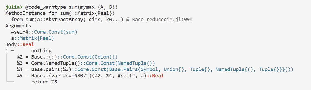
# 使用 @code_warntype 检测类型稳定

使用@code_warntype宏可以帮助诊断类型稳定。

例如，针对前面的类型不稳定示例，在 Julia 命令行窗口输入@code_warntype sum(mymax.(A, B))，显示类型推断结果。其中红色高亮表示告警，即存在类型不稳定。

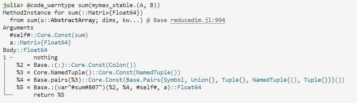
针对前面的类型稳定示例，在 Julia 命令行窗口输入@code_warntype sum(mymax_stable.(A, B))，没有出现红色高亮告警，即表示是类型稳定的。

# 避免使用抽象类型参数的容器

相比于Any、Number等抽象类型，使用Int、Float64等具体类型可以带来更好的性能。数据类型越具体，编译器就越有可能给出好的优化策略。

示例 1：

a是一个抽象类型Real的数组，所以它能够保存任何Real值。由于Real对象允许具有任意大小和结构，因此a必须表示为指向单独分配的Real对象的指针数组。

b是一个具体类型Float64的数组，按照 64 位浮点数值的连续的块来储存，更能高效地处理。

using BenchmarkTools

# 抽象数据类型
a = []
@btime begin
    push!(a,1);push!(a,2.0);push!(a,pi);
end
# 101.921 ns (0 allocations: 0 bytes)

# 具体数值类型
b = Float64[]
@btime begin
    push!(b,1);push!(b,2.0);push!(b,pi);
end
# 47.273 ns (0 allocations: 0 bytes)

示例 2：

生成一个元素为Any类型的矩阵A，生成一个元素为Int类型的矩阵B：

A = Matrix(undef,10,10);
B = Matrix{Int}(undef,10,10);

A、B赋值为 10 阶幻方矩阵：

using TyMath
A .= magic(10);
B .= magic(10);

用@btime去测试对A、B求和的时间：

using BenchmarkTools
@btime sum($A)  # 1.380 μs (90 allocations: 1.41 KiB)
@btime sum($B)  # 7.900 ns (0 allocations: 0 bytes)

# 结构体的类型声明应该尽可能具体

结构体的类型声明也应该尽可能是具体的。

在没有类型标记的情况下，结构体元素类型为Any。性能测试如下：

struct Point2D
    x # 不标注类型，默认为 Any 类型
    y # 不标注类型，默认为 Any 类型
end

gen_points(n) = [Point2D(rand(), rand()) for i in 1:n]

dist(x::Point2D, y::Point2D) = sqrt((x.x - y.x)^2 + (x.y - y.y)^2)

function f_dist(points)
    p = Point2D(0.0, 0.0)
    n = length(points)
    out = Vector{Float64}(undef, n)
    for i in 1:n
        out[i] = dist(p, points[i])
    end
    return out
end

points = gen_points(1024)

using BenchmarkTools
@btime f_dist($points) # 104.200 μs (6658 allocations: 112.14 KiB)

对于本示例，将声明结构体的元素类型指定具体类型，其余保持不变，性能会大幅提升。

注意

用户自行比较时，需要重启命令行窗口，否则易出现重定义报错。

struct Point2D
    x::Float64 # 指定具体类型
    y::Float64 # 指定具体类型
end

# 其余代码保持不变
gen_points(n) = [Point2D(rand(), rand()) for i in 1:n]

dist(x::Point2D, y::Point2D) = sqrt((x.x - y.x)^2 + (x.y - y.y)^2)

function f_dist(points)
    p = Point2D(0.0, 0.0)
    n = length(points)
    out = Vector{Float64}(undef, n)
    for i in 1:n
        out[i] = dist(p, points[i])
    end
    return out
end

points = gen_points(1024)

using BenchmarkTools
@btime f_dist($points) # 1.380 μs (1 allocation: 8.12 KiB)

# 内存优化

# 数组预分配

如果函数返回Array或其它复杂类型，则可能需要分配内存。

# bad
function test_bad(b::Vector{Int})
    a = Int[]
    n = length(b)
    @inbounds for i in 1:n
        push!(a,b[i])
    end
    return a
end

如果在数组大小已知的情况下，可以提前分配内存，可以大幅提升效率。

# good
function test_good(b::Vector{Int})
    n = length(b)
    a = Vector{Int}(undef, n)
    @inbounds for i in 1:n
        a[i] = b[i]
    end
    return a
end

两者性能对标如下：

using TyRandom
b = randi(10, 1000) # 1~10之间的随机整数向量

using BenchmarkTools
@btime test_bad($b); # 4.333 μs (6 allocations: 21.86 KiB)
@btime test_good($b); # 357.732 ns (1 allocation: 7.94 KiB)

# 数组切片使用视图

在 Julia 中，像array[1:5, :]这样的数组“切片”表达式会创建该数据的副本（赋值的左侧除外，其中array[1:5, :] = ...原地对array的那一部分进行赋值）。另一种方法是创建数组的“视图”，它实际上就地引用了原始数组的数据，而不进行复制。如果你写入视图，它也会修改原始数组的数据。

例如，x是一个数组，v = @view x[1:10]，则v表现得就像一个含有 10 个元素的数组，但是它的数据实际上是访问x的前 10 个元素。对视图的写入，如v[3] = 2，直接写入了底层的数组x（这里是修改x[3]）。

x = rand(100)
v = @view x[1:10]
v[3] = 2 # 原始数组的数据也会被修改
x[3] == 2 # true

@views宏可以用于整个代码块（如@views function foo() .... end或@views begin ... end）来将整个代码块中的切片操作变为使用视图。

fcopy(x) = sum(x[2:end])
@views fview(x) = sum(x[2:end])

x = rand(10^6)

using BenchmarkTools
@btime fcopy(x); # 1.375 ms (3 allocations: 7.63 MiB)
@btime fview(x); # 133.400 μs (1 allocation: 16 bytes)

# 避免中间结果的矩阵创建

避免中间结果的矩阵创建，可以明显提升代码性能。

例如，对一个矩阵元素的绝对值求和，abs.(A)会创建一个中间矩阵。

A = rand(1024,1024) .- 0.5

using BenchmarkTools
@btime sum(abs.(A)) # 1.763 ms (5 allocations: 8.00 MiB)
@btime sum(abs, A) # 142.700 μs (1 allocation: 16 bytes)

sum(abs, A)不会创建中间矩阵，其实现过程大致为：

function sumabs(A)
    rst = zero(eltype(A))
    @simd for x in A
        rst += abs(x) # 实际上 abs 的中间结果只需用标量表示
    end
    return rst
end

@btime sumabs(A) # 139.000 μs (1 allocation: 16 bytes)

Julia 存在非常多高阶函数，如map, reduce, sum, mean等，用于避免手写循环。

# 数组拷贝与共享

Julia 提供了很多数组相关的操作函数，其中有些是拷贝，有些是引用（即共享底层数据）。

例如，我们可以使用 vec 或 [:] 将矩阵转为向量，如下所示：

生成矩阵A：

A = rand(100,100);

将矩阵A转为向量形式，并测试性能。

using BenchmarkTools
@btime vec(A); # 28.141 ns (2 allocations: 80 bytes)
@btime A[:]; # 2.587 μs (2 allocations: 78.17 KiB)

可以看出，vec 效率更高，原因是 vec 不拷贝数组，而是共享底层数据。

为了方便大家使用，我们对一些典型的数组使用场景进行梳理，如下表所示。

使用场景	说明	举例
数组赋值	共享底层数据	`a = [1,2,3]` `b = a` `a[1] = 10` `b # 输出：[10, 2, 3]`
数组切片	拷贝	`a = [1 2 3;4 5 6]` `b = a[1,:]` `a[1] = 10` `b # 输出：[1, 2, 3]`
数组视图 @view	共享底层数据	`a = [1 2 3;4 5 6]` `b = @view a[1,:]` `a[1] = 10` `b # 输出：[10, 2, 3]`
reshape	共享底层数据	`a = [1,2,3,4]` `b = reshape(a, 2, 2)` `a[1] = 10` `b # 输出：[10 3; 2 4]`
collect	拷贝	`a = [1,2,3,4]` `b = collect(a)` `a[1] = 10` `b # 输出：[1, 2, 3, 4]`
vec	共享底层数据	`a = [1 2; 3 4]` `b = vec(a)` `a[1] = 10` `b # 输出：[10, 3, 2, 4]`
共轭转置：', adjoint	共享底层数据	`a = [3+2im 9+2im; 0 0]` `b = a'` `a[1] = 10` `b # 输出：[10+0im 0; 9-2im 0]`
转置：transpose	共享底层数据	`a = [3+2im 9+2im; 0 0]` `b = transpose(a)` `a[1] = 10` `b # 输出：[10+0im 0; 9+2im 0]`
实数共轭：conj	共享底层数据	`a=[1 2 ;3 4]` `b=conj(a)` `a[1] = 10` `b # 输出：[10 2; 3 4]`
复数共轭：conj	拷贝	`a = [3+2im 9+2im; 0 0]` `b = conj(a)` `a[1] = 10` `b # 输出：[3-2im 9-2im; 0 0]`

# inplace 原地操作

在 Julia 中，in-place（原地）操作指的是直接修改输入对象本身，而不是创建并返回一个新的对象。这种操作可以避免不必要的内存分配（尤其是对大型数据结构，如数组），从而提升性能，是 Julia 中优化代码效率的重要手段。

Julia 中约定：函数名末尾带有感叹号 ! 的函数，通常是 in-place 操作，会修改至少一个输入参数。这个 ! 只是命名约定（不是语法），但它清晰地向开发者传递了 “此函数会修改输入” 的信息，提高代码可读性。

例如，在连续的向量拼接过程中，可以使用 push! 或 append!（append! 是添加向量，push! 是添加标量）替代 [a;b] 或 vcat(a,b)，因为使用 push 或 append 后，数组会有缓冲区，不会频繁产生复制，而 vcat 的方式总会发生复制，频繁的复制在循环中会造成很大的开销。

x = Float64[]
y = Float64[]

n = 100_000

# good
function func_fast(x, n)
    for i in 1:n
        push!(x, i) # 原地操作
    end
    return x
end

# bad
function func_slow(y,n)
    for i in 1:n
        y = [y;i] # 或 vcat(y,i)
    end
    return y
end

@time func_fast(x,n)      # 0.006454 seconds (2.47 k allocations: 1.994 MiB)
@time y = func_slow(y, n) # 11.973289 seconds (200.62 k allocations: 37.261 GiB, 17.10% gc time)

x == y # true

# 高阶函数的使用

在 Julia 中，高阶函数（Higher-Order Functions） 是指能够接受其他函数作为参数，或返回一个函数作为结果的函数。这种特性是函数式编程的核心，能极大地提高代码的抽象能力和复用性。Julia 内置了许多实用的高阶函数，同时也允许用户自定义高阶函数。

例如，all 函数用于检查所有元素是否满足某个条件，其定义为all(Function, data)形式。

生成向量A，其中前 1000 个数为整数，后 1000 个数为非整数：

using TyRandom
A = [randi(1000,1000);rand(1000)]

分别使用两种方式计算并用@btime测试时间：

using BenchmarkTools
@btime all(isinteger.(A)); # 885.000 ns (5 allocations: 4.58 KiB)
@btime all(isinteger, A); # 638.788 ns (0 allocations: 0 bytes)

使用all(Function, data)形式，可减少内存消耗，同时可以利用短路效应提前返回。

提示

提供相关接口的函数还有sum,mean,median,findall,findfirst,findlast,maximum,minimum,any等等。

# 使用 UnitRange 索引效率更高

生成Vector和UnitRange两种类型的索引：

ind1 = 1:10_000;
ind2 = collect(ind1);

typeof(ind1) # UnitRange{Int64}
typeof(ind2) # Vector{Int64}

测试使用两种类型索引的效率。可以看出，使用UnitRange索引效率更高。

a = rand(100_000)

using BenchmarkTools
@btime a[ind1]; # 2.725 μs (2 allocations: 78.17 KiB)
@btime a[ind2]; # 4.925 μs (2 allocations: 78.17 KiB)

# 循环优化

# 沿列按内存顺序访问数组

在一门足够高性能的语言中（C/C++、Julia），内存是高性能计算必须要考虑的因素。CPU 在处理内存中的数据（矩阵）的时候，会先将数据读取到 CPU 缓存中。CPU 在从内存中加载缓存的时候，每次会加载一段连续的内存而非单个值。沿着数组的内存排列顺序使用矩阵，缓存命中率更高。

Julia 中的多维数组以列主序存储。例如：

A = [1 3; 2 4]
#=
2×2 Matrix{Int64}:
 1  3
 2  4
=#

A[:]
#=
4-element Vector{Int64}:
 1
 2
 3
 4
=#

沿行的方向进行迭代：

# bad
function mysum_rowwise(A)
    rst = zero(eltype(A))
    for i in axes(A, 1)
        for j in axes(A, 2)
            rst += A[i,j]
        end
    end
    return rst
end

沿列的方向进行迭代：

# good
function mysum_colwise(A)
    rst = zero(eltype(A))
    for j in axes(A, 2)
        for i in axes(A, 1)
            rst += A[i,j]
        end
    end
    return rst
end

两者性能比较：

A = rand(1024, 512)
using BenchmarkTools
@btime mysum_rowwise(A) # 855.600 μs (1 allocation: 16 bytes)
@btime mysum_colwise(A) # 429.000 μs (1 allocation: 16 bytes)

# 使用 @inbounds 与 @simd 加速 for 循环

有时，可以通过承诺某些程序性质来启用更好的优化。

使用@inbounds来取消表达式中的数组边界检查。使用前请再三确定，如果下标越界，可能会发生崩溃或潜在的故障；
在 for 循环前编写@simd来承诺迭代是相互独立且可以重新排序的。此外，在断言@simd时要十分小心，因为错误地标注一个具有相互依赖的迭代的循环可能导致意外结果。

不使用性能标注，示例如下：

@noinline function inner(x, y)
    s = zero(eltype(x))
    for i = eachindex(x)
        s += x[i]*y[i]
    end
    return s
end

使用性能标注，示例如下：

@noinline function inner_simd(x, y)
    s = zero(eltype(x))
    @simd for i = eachindex(x) # 前提条件：SIMD 需要顺序无关的循环
        @inbounds s += x[i] * y[i]
    end
    return s
end

两者性能比较，可以看出性能标注可以大幅提升性能。

x = rand(1000)
y = rand(1000)

using BenchmarkTools
@btime inner(x,y) # 861.111 ns (1 allocation: 16 bytes)
@btime inner_simd(x,y) # 78.395 ns (1 allocation: 16 bytes)

# 使用 ifelse 函数消除条件分支，用于支持 SIMD

在 Julia 中，@simd宏的作用是向编译器提示循环体内的迭代是独立的，可以被安全地重新排序。这使得编译器可以自由地使用 SIMD 指令（单指令多数据流）来并行执行循环体内的操作，从而提高运行时性能。

根据经验来看，使用 SIMD 需要满足：

需要不中断的固定长度循环
- 循环长度预先指定
- 循环体内不存在分支（即if语句）
需要顺序无关的循环

例如，for 循环体内存在条件分支，@simd不生效。

# @simd 不生效
function test_if(y)
    _1_, _0_ = one(eltype(y)), zero(eltype(y))
    @simd for i in eachindex(y)
        yi = y[i]
        if yi < 0
            y[i] = _0_
        elseif yi > 1
            y[i] = _1_
        end
    end
    return y
end

可以采用ifelse函数来消除分支语句，从而使得@simd生效。

# @simd 生效
function test_simd(y)
    _1_, _0_ = one(eltype(y)), zero(eltype(y))
    @simd for i in eachindex(y)
        yi = y[i]
        y[i] = ifelse(yi < _0_, _0_, ifelse(yi > _1_, _1_, yi))
    end
    return y
end

两者性能对比：

x=(rand(64, 64) .- 0.5) .* 5

using BenchmarkTools
@btime test_if(x); # 723.810 ns (0 allocations: 0 bytes)
@btime test_simd(x); # 236.658 ns (0 allocations: 0 bytes)

# 使用 Threads.@thread 多线程加速

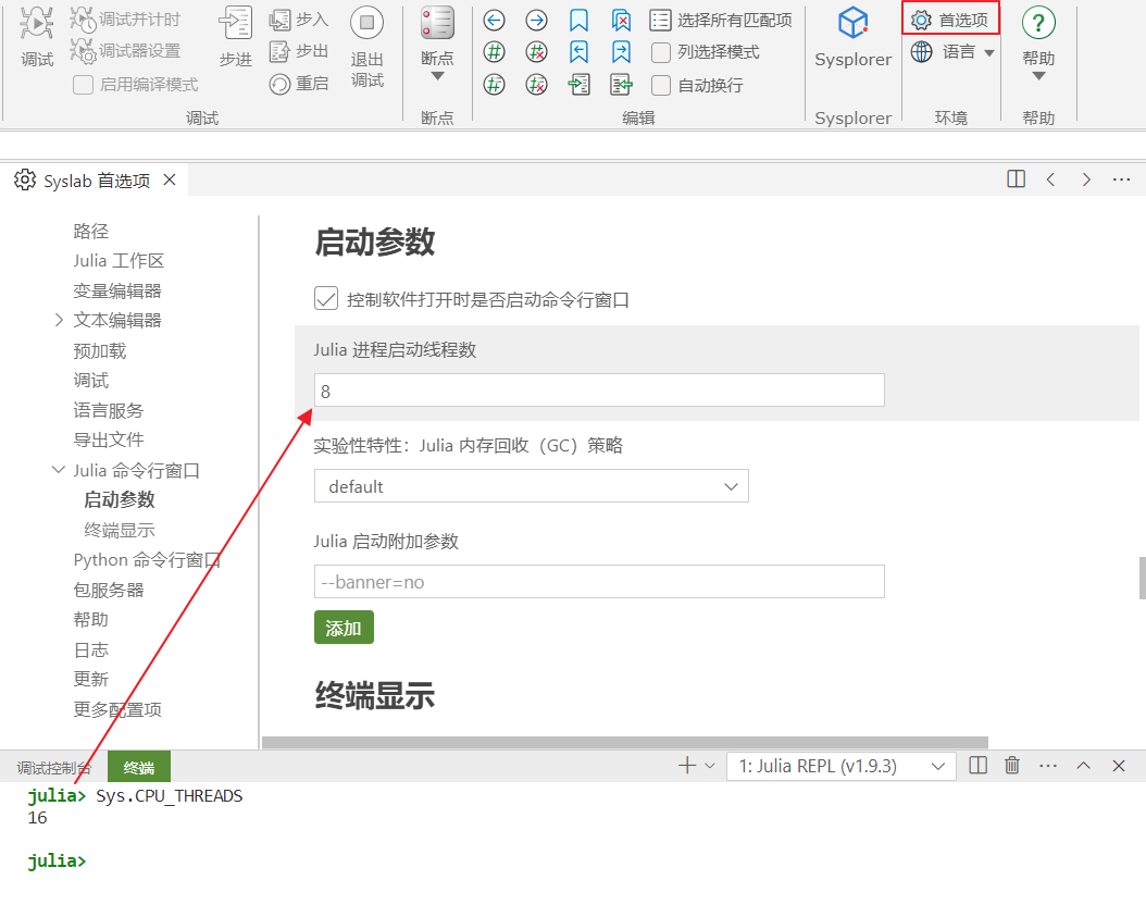
Julia 提供了丰富的并行计算能力，包括异步计算、多线程计算、多进程计算、GPU 及异构计算。其中，多现场计算使用较为普遍。在使用多线程加速前，设置 Julia 启动线程数，一般推荐设置为计算机线程数的一半。

首先，打开 Syslab，在 Julia 命令行窗口中输入Sys.CPU_THREADS可以查看计算机线程数；其次，打开首选项页面，设置 Julia 启动线程数，一般设置为计算机线程数的一半，设置完成后需要重启命令行窗口生效。

通过在 for 循环前面添加Threads.@threads，即可将其变成多线程执行代码。

注意：使用多线程并行加速，要求每个线程的迭代操作相互独立，避免数据竞争。

using TyPlot
using TyImageProcessing
using BenchmarkTools

# 加载图像
img = imread("corn.tif");
h, w = size(img)

# 预分配内存
gray_img = Matrix{Float64}(undef, h, w)
gray_img2 = similar(gray_img)

# 使用多线程
@btime Threads.@threads for i in 1:h
    for j in 1:w
        # 获取原图像素
        pixel = img[i, j, :] ./ 255

        # 计算灰度值（每个线程操作不同位置，无竞争）
        gray_img[i, j] = 0.299 * pixel[1] + 0.587 * pixel[2] + 0.114 * pixel[3]
    end
end

# 不使用多线程
@btime for i in 1:h
    for j in 1:w
        # 获取原图像素
        pixel = img[i, j, :] ./ 255

        # 计算灰度值（每个线程操作不同位置，无竞争）
        gray_img2[i, j] = 0.299 * pixel[1] + 0.587 * pixel[2] + 0.114 * pixel[3]
    end
end

gray_img == gray_img2 # true

# 使用多线程：  18.251 ms (1683707 allocations: 47.43 MiB)
# 不使用多线程：104.305 ms (1684071 allocations: 47.44 MiB)

关于 Julia 并行计算能力，详细请参阅 Syslab 帮助文档的并行计算工具箱。

# 合理使用广播和向量化编程

# 合理使用点运算符

为了便于数学上和其他运算的向量化，Julia 提供了点语法，如sin.(x)，用于数组或数组和标量的混合上的按元素运算（广播运算）。在 Julia 中，广播与 for 循环的行为与性能是一致的。

合理使用点运算符，对于标量情况，无需加点操作符。

定义一个标量a：

a = 10;

通过加点操作符和不加点操作符，对a做 10000 次平方操作：

using BenchmarkTools

# bad
@btime for i in 1:10000
        a .^ 2
end
# 7.678 ms (50000 allocations: 1.07 MiB)

# good
@btime for i in 1:10000
        a ^ 2
end
# 94.000 μs (0 allocations: 0 bytes)

# 广播赋值

对于数组来说，使用.=或类似的赋值运算符，运算结果可以原地（in-place）存储在预分配的数组，节省内存开销。

例如：

using TyMath

# bad
function foo1()
    rng=MT19937ar(5489)
    a =randn(rng,1000)
    for ii in 1:100000
        t = randi(rng,(0,ii),1000)
        a += sin.(t)
    end
    return a
end

# good
function foo2()
    rng=MT19937ar(5489)
    a =randn(rng,1000)
    for ii in 1:100000
        t = randi(rng,(0,ii),1000)
        a .+= sin.(t) # 广播赋值
    end
    return a
end

using BenchmarkTools
@btime foo1() # 3.226 s (300003 allocations: 2.27 GiB)
@btime foo2() # 3.041 s (100003 allocations: 775.16 MiB)

不难发现，通过逐元素（element-wise）的广播赋值，我们减少了 2/3 的内存分配。究其原因，.+=采用原地赋值（即运算结果仍在原数组内存地址上），而+=会重新分配内存。

那么，如何知道数组内存地址发生改变，做个小测试：

a = randn(10)
addr1 = pointer_from_objref(a)
# Ptr{Nothing} @0x000001a090088520

a .+= 1:10
addr2 = pointer_from_objref(a)
# Ptr{Nothing} @0x000001a090088520

a += 1:10
addr3 = pointer_from_objref(a)
# Ptr{Nothing} @0x000001a09379f460

可以看到，.+=操作后原数组的 pointer 并没有改变。而+=操作后，原数组的 pointer 改变了，说明对于数组的+=来说，会在新的内存地址中重新赋值。

# 合理使用广播

使用广播向量化地编程，能够使代码更简洁并且性能也不会受太多影响。但是在部分场景中，广播的使用需要慎重，尤其是大型数组的运算中。

Julia 的点语法，可以将任何标量函数转换为「向量化」函数调用，可以将任何运算符转换为「向量化」运算符。它具有的特殊性质是嵌套「点调用」是融合的：它们在语法层级被组合为单个循环，无需分配临时数组。如果你使用.=和类似的赋值运算符，则结果也可以 in-place 存储在预分配的数组（参见上文）。

在线性代数的上下文中，这意味着即使诸如vector + vector和vector * scalar之类的运算，使用vector .+ vector和vector .* scalar来替代也可能是有利的，因为生成的循环可与周围的计算融合。

例如：

using TyMath
a = 3/pi

rng=MT19937ar(5489)
b =randn(rng,10^6)
c =randn(rng,10^6)

using BenchmarkTools
@btime sin(a) * b + cos(a) * c # 4.332 ms (8 allocations: 22.89 MiB)

我们可以采用@.宏对上述表达式进行向量化编程。

# bad
@btime @. sin(a) * b + cos(a) * c; # 9.235 ms (12 allocations: 7.63 MiB)
@btime sin.(a) .* b .+ cos.(a) .* c; # 9.185 ms (12 allocations: 7.63 MiB)，等价于上句

不难发现，虽然内存分配减少了 2/3，但是性能反而恶化了。原因是@. sin(a) * b + cos(a) * c等价于sin.(a) .* b .+ cos.(a) .* c，在每次的循环中都对sin(a)、cos(a)进行重复计算，从而导致效率下降。

原因清楚了，接下来我们需要引入变量来避免重复计算，代码如下：

# good
sin_a = sin(a)
cos_a = cos(a)
@btime @. sin_a * b + cos_a * c; # 1.335 ms (8 allocations: 7.63 MiB)
@btime sin_a .* b .+ cos_a .* c; # 1.319 ms (8 allocations: 7.63 MiB)，等价于上句

因此，广播的使用需要特别小心，尽量避免标量的重复计算。如果遇到不确定的地方，可以在使用时先尝试一下。

# 使用高效的算法和数据结构

# 使用 Tuple 或 NamedTuple 来代替 Vector 或 Dict

数组是可变类型，在堆上分配内存；元组（Tuple）是不可变类型，在栈上分配内存。相比于堆内存，栈内存具有更高的内存分配与使用效率。因此，在某些场景下，可以使用Tuple或 NamedTuple 来代替Vector或Dict。

注意

元组是不可修改的，元组的修改往往表现为创建一个新的元组。

例如：

function mysum(pairs)
    r1, r2 = 0.0, 0.0
    @simd for p in pairs
        r1 += p[1]
        r2 += p[2]
    end
    return r1,r2
end

using BenchmarkTools

# 使用 Vector
pairs = [[rand(), rand()] for _ in 1:1024]
@btime mysum(pairs) # 860.714 ns (1 allocation: 32 bytes)

# 使用 Tuple
pairs = [(rand(), rand()) for _ in 1:1024]
@btime mysum(pairs) # 228.995 ns (1 allocation: 32 bytes)

# clamp! 将数组中的值限制在某个区间内

clamp!函数用于将数组中的值限制在指定范围的适当位置内。其声明为：

clamp!(array::AbstractArray, lo, hi)

例如，把数组的值限制在 0 到 1 之间，两种实现方式：

# bad
function test1(y)
    _1_, _0_ = one(eltype(y)), zero(eltype(y))
    for i in eachindex(y)
        if y[i] < _0_
            y[i] = _0_
        elseif y[i] > _1_
            y[i] = _1_
        end
    end
    return y
end

# good
function test2(y)
    _1_, _0_ = one(eltype(y)), zero(eltype(y))
    return clamp!(y, _0_, _1_)
end

通过两者性能对比，发现clamp!性能更高。

using BenchmarkTools
@btime test1(x) setup=(x=(rand(64, 64) .- 0.5) .* 5); # 725.373 ns
@btime test2(x) setup=(x=(rand(64, 64) .- 0.5) .* 5); # 255.000 ns

提示

clamp!会直接改变元数据，而@btime是多次执行的，因此直接做@btime f(x)的话会导致它测试的实际上是一个已经被修正过的数据，结果是分支预测永远正确时的性能（过于理想）。此处使用@btime的setup设置，保证了每次测试的数据为新生成的数据。

# 有序数组查找

在确认查找的数组为有序数组时，使用searchsortedlast函数要比findlast函数有更好的性能：

定义一个长度为 1000000 的数组，并排序:

a = rand(1000000)
sort!(a)

使用两种函数，并使用@btime测试时间：:

using BenchmarkTools
@btime findlast(<=(0.9),a) # 42.500 μs (2 allocations: 32 bytes)
@btime searchsortedlast(a,0.9) # 44.848 ns (1 allocation: 16 bytes)

# 整数求整除部分时，可以使用 div

有两种方式计算整除：

a = 5;
b = 2;

using BenchmarkTools

# bad
@btime for i in 1:10000
    floor(Int, a / b)
end
# 832.200 μs (10000 allocations: 156.25 KiB)

# good
@btime for i in 1:10000
    div(a, b)
end
# 104.600 μs (0 allocations: 0 bytes)

提示

div(a,b)等价于a÷b，÷键入\div可打出。

# 矩阵求逆的推荐写法

对于矩阵求逆，a * inv(b)更推荐的写法是a/b，同理inv(a) * b更推荐使用a\b去做，MATLAB 也是更推荐这种语法，性能会更高。

a = rand(100,100)
b = rand(100,100)

using BenchmarkTools
@btime a * inv(b) # 1.537 ms (7 allocations: 207.34 KiB)
@btime a/b # 1.246 ms (7 allocations: 235.39 KiB)

同理，

@btime inv(a)*b # 1.542 ms (7 allocations: 207.34 KiB)
@btime a\b # 1.213 ms (5 allocations: 157.22 KiB)

# 判空尽量使用 isempty 函数

字符串、向量等判断是否为空，尽量使用isempty函数，性能更优。

a=[1,2,3]

using BenchmarkTools
@btime isempty(a) # 11.712 ns (0 allocations: 0 bytes)
@btime length(a)==0 # 22.066 ns (0 allocations: 0 bytes)